Waveform Arithmetic
There are three types of mathematical operations that can be performed on waveform data:
1. Plot expressions of traces.
2. Compute the average or RMS of a trace.
3. Display the Fourier Transform of a trace.
1. Plot expressions of traces.
Both the View=>Visible Traces and View=>Add Trace commands allow one to enter an expression of data. Another method to plot an expression of available simulation data traces is to move the mouse to the trace's label and right click. This dialog box also allows you to set the trace's color and allows you to attach a cursor to the waveform. LTspice will do a dimensional analysis of the expression and plot it against a vertical axis labeled with those units. For example, below you can see that LTspice identified the dimensions of -2*p*pow(V(out),2)/abs(V(n001))/Ie(x1:Q1) as Ω. All waveforms in a plotting pane with the same units are plotted on the same axis.

The difference of two voltages; e.g., V(a)-V(b); can written equivalently as V(a,b). The following functions are available for real data:
| Function Name | Description |
| abs(x) | Absolute value of x |
| acos(x) | Arc cosine of x |
| arccos(x) | Synonym for acos() |
| acosh(x) | Arc hyperbolic cosine |
| asin(x) | Arc sine of x |
| arcsin(x) | Synonym for sin() |
| asinh(x) | Arc hyperbolic sine |
| atan(x) | Arc tangent of x |
| arctan(x) | Synonym for atan() |
| atan2(y,x) | Four quadrant arc tangent of y/x |
| atanh(x) | Arc hyperbolic tangent |
| buf(x) | 1 if x > .5, else 0 |
| ceil(x) | Integer equal or greater than x |
| cos(x) | Cosine of x |
| cosh(x) | Hyperbolic cosine of x |
| d() | Finite difference-based derivative |
| exp(x) | e to the x |
| floor(x) | Integer equal to or less than x |
| hypot(x,y) | sqrt(x**2 + y**2) |
| if(x,y,z) | If x > .5, then y else z |
| int(x) | Convert x to intege |
| inv(x) | 0. if x > .5, else 1. |
| limit(x,y,z) | Intermediate value of x, y, and z |
| ln(x) | Natural logarithm of x |
| log(x) | Alternate syntax for ln() |
| log10(x) | Base 10 logarithm |
| max(x,y) | The greater of x or y |
| min(x,y) | The smaller of x or y |
| pow(x,y) | x**y |
| pwr(x,y) | abs(x)**y |
| pwrs(x,y) | sgn(x)*abs(x)**y |
| rand(x) | Random number between 0 and 1 depending on the integer value of x. |
| random(x) | Similar to rand(), but smoothly transitions between values. |
| round(x) | Nearest integer to x |
| sgn(x) | Sign of x |
| sin(x) | Sine of x |
| sinh(x) | Hyperbolic sine of x |
| sqrt(x) | Square root of x |
| table(x,a,b,c,d,...) | Interpolate a value for x based on a look up table given as a set of pairs of points. |
| tan(x) | Tangent of x. |
| tanh(x) | Hyperbolic tangent of x |
| u(x) | Unit step, i.e., 1 if x > 0., else 0. |
| uramp(x) | x if x > 0., else 0. |
| white(x) | Random number between -.5 and .5 smoothly transitions between values even more smoothly than random(). |
For complex data, the functions atan2(,), sgn(), u(), buf(), inv() uramp(), int(), floor(), ceil(), rand(), min(,), limit(,), if(,,), and table(...) are not available. The functions Re(x) and Im(x) are available for complex data and return a complex number with the real part equal to the real or imaginary part of the argument respectively and the imaginary part equal to zero. The functions Ph(x) and Mag(x) are also available for complex data and return a complex number with the real part equal to the phase angle or magnitude of the argument respectively and the imaginary part equal to zero. The function conj(x) is also available for complex data and returns the complex conjugate of x.
The following operations, grouped in reverse order of precedence of evaluation, are available for real data:
| Operand | Description |
| & | Convert the expressions to either side to Boolean, then AND. |
| | | Convert the expressions to either side to Boolean, then OR. |
| ^ | Convert the expressions to either side to Boolean, then XOR. |
| > | TRUE if expression on the left is greater than the expression on the right, otherwise FALSE. |
| < | TRUE if expression on the left is less than the expression on the right, otherwise FALSE. |
| >= | TRUE if expression on the left is greater than or equal the expression on the right, otherwise FALSE. |
| <= | TRUE if expression on the left is less than or equal the expression on the right, otherwise FALSE. |
| + | Addition |
| - | Subtraction |
| * | Multiplication |
| / | Division |
| ** | Raise left hand side to power of right hand side. |
| ! | Convert the following expression to Boolean and invert. |
| @ | Step selection operator |
TRUE is numerically equal to 1 and FALSE is 0. Conversion to Boolean converts a value to 1 if the value is greater than 0.5, otherwise the value is converted to 0.
The step selection operator, '@' is useful when multiple simulation runs are available as in a .step, .temp, or .dc analysis. It selects the data from a specific run. For example, V(1)@3 would plot the data from the 3rd run no matter what steps where selected for plotting.
For complex data, only +, -, *, /, **, and @ are available. Also with regard to complex data, the Boolean XOR operator, ^ is understood to mean exponentiation, **.
The following constants are internally defined:
| Name | Value |
| E | 2.7182818284590452354 |
| pi | 3.14159265358979323846 |
| K | 1.3806503e-23 |
| Q | 1.602176462e-19 |
The keyword "time" is understood when plotting transient analysis waveform data. Similarly, "freq" and "omega" are understood when plotting data from an AC analysis. "w" can be used as a synonym for omega.
2. Compute the average or RMS of a trace.
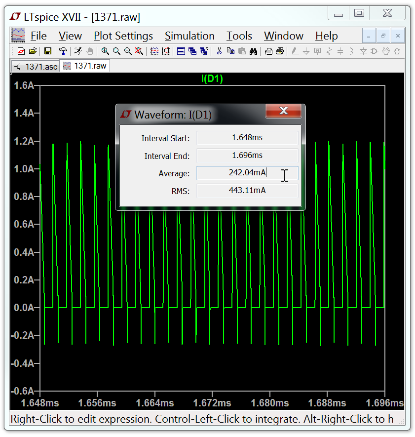
The waveform viewer can integrate a trace to obtain the average and RMS value over the displayed region. First zoom the waveform to the region of interest, then move the mouse to the label of the trace, hold down the control key and left mouse click.

Note RMS average is reported only if the physical units of the integrated quantity is volts or amps to avoid confusing people that need the average when power is integrated.
3. Display the Fourier Transform of a Trace.
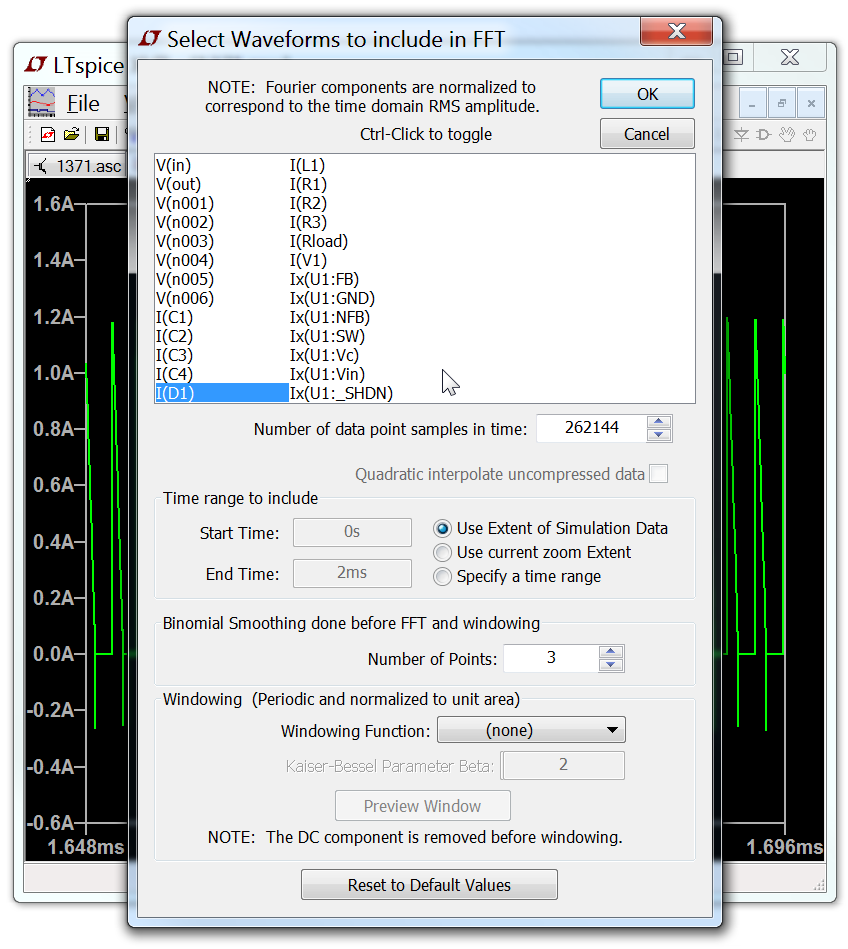
You can use the menu command View=>FFT to perform a Fast Fourier transform on various data traces.

LTspice uses a proprietary FFT algorithm that allows an arbitrary number of datapoints, i.e., not limited to a power of 2.
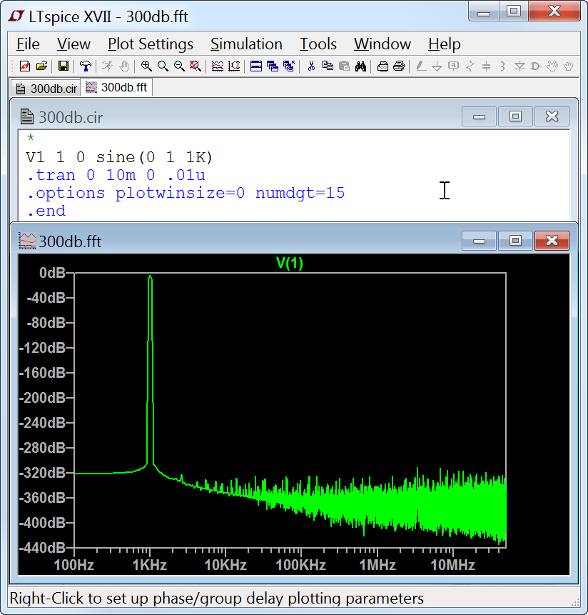
When you expect to do FFT's of your simulation data, you will probably want to turn off waveform compression, stipulate a maximum time step, and possibly even use double precision waveform file format to reduce the numeric noise floor. The following netlist shows that the intrinsic noise floor of LTspice's FFT algorithm is in excess of 300dB.
